

In statistical hypothesis testing, every research question is formalized into two competing, mutually exclusive statements: the null hypothesis (H₀), which represents “no effect” or “no difference,” and the alternative hypothesis (H₁ or Hₐ), which represents the effect or difference the researcher is actually investigating. The entire logic of statistical testing is built around these two — you don’t directly prove your research hypothesis; you test whether the evidence is strong enough to reject the null in its favor.
Why Hypothesis Testing Is Built Around “Failing to Reject,” Not “Proving”
This is the single most important conceptual point in the entire topic, and it’s frequently stated backward in casual writing. Statistical tests never prove the alternative hypothesis is true. They assess whether the observed data would be unusually unlikely if the null hypothesis were actually true — and if so, the null is rejected in favor of the alternative. If the data isn’t unusual enough, you fail to reject the null — which is not the same as proving the null is true.
This asymmetry matters: absence of evidence against H₀ is not evidence that H₀ is correct — it may simply mean the study lacked the statistical power to detect a real effect that does exist.
Formal Definitions and Notation
Null hypothesis (H₀): a statement of no effect, no relationship, or no difference between groups — the default assumption that any observed pattern in the data is due to random chance alone.
Alternative hypothesis (H₁ or Hₐ): a statement that there is an effect, relationship, or difference — this is typically what the researcher’s actual research question is trying to establish evidence for.
Critically, H₀ and H₁ must be mutually exclusive and collectively exhaustive — together they must cover every possible outcome, with no overlap.
Worked Example 1: A Two-Sample Comparison
Research question: Does a new teaching method improve exam scores compared to the standard method?
H₀: μ_new = μ_standard   (no difference in mean exam scores)
H₁: μ_new ≠ μ_standard   (there is a difference in mean exam scores)
Here, μ represents the population mean score for each group. Note that H₁ simply states “not equal” — it doesn’t yet specify a direction (this is a two-tailed hypothesis, covered below).
Worked Example 2: A Directional (One-Tailed) Hypothesis
Research question: Does the new teaching method specifically improve exam scores (not just change them in either direction)?
H₀: μ_new ≤ μ_standard   (new method does not improve scores)
H₁: μ_new > μ_standard   (new method improves scores)
This is a one-tailed (directional) hypothesis, since H₁ specifies a particular direction of effect, not just “some difference exists.”
One-Tailed vs Two-Tailed Tests: Why the Distinction Matters
This distinction directly affects how the test is conducted and interpreted, particularly regarding where the “rejection region” sits on the underlying probability distribution.
- Two-tailed test: H₁ states the parameter is simply different from the null value, without specifying direction. The rejection region is split across both tails of the distribution.
- One-tailed test: H₁ specifies a direction (greater than or less than). The entire rejection region sits in a single tail, corresponding to that direction.
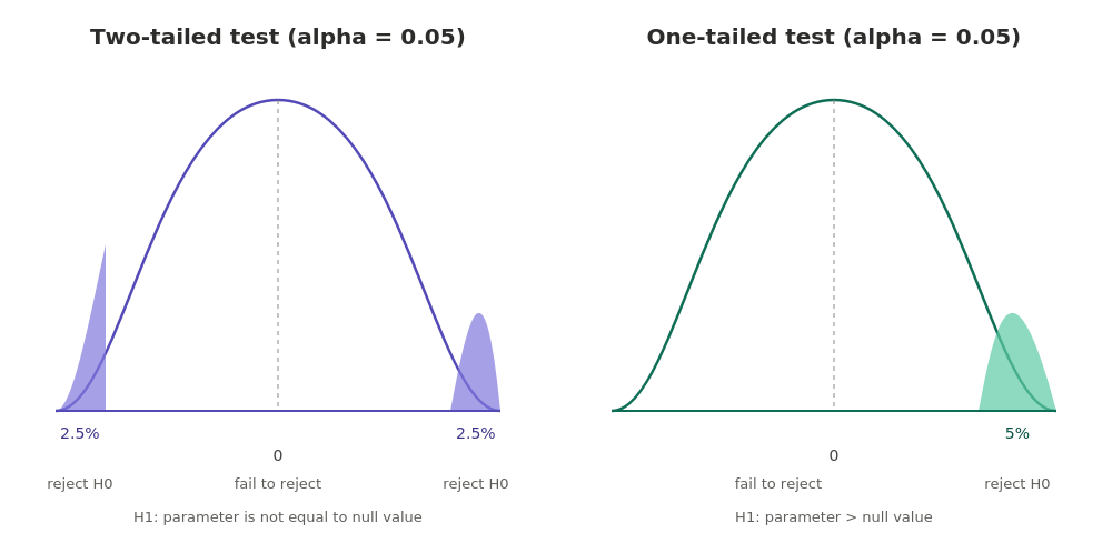
A common and consequential student error is running a two-tailed test but interpreting the results as though it were one-tailed (or vice versa) — this changes the critical value and can lead to incorrectly rejecting or failing to reject H₀. The choice between one-tailed and two-tailed must be decided before looking at the data, based on the actual research question — deciding afterward, based on which direction the data happened to trend, is a form of data-driven bias that invalidates the test’s statistical logic.
The Decision Framework: Connecting to the P-value
Hypothesis testing formalizes the decision using a significance threshold, typically α = 0.05:
- Assume H₀ is true
- Calculate a test statistic from the sample data
- Determine the p-value — the probability of observing data this extreme (or more extreme) if H₀ were actually true
- If p ≤ α: reject H₀ in favor of H₁ (the result is “statistically significant”)
- If p > α: fail to reject H₀ (insufficient evidence to conclude an effect exists)
Worked example continuing the teaching method study: Suppose the one-tailed test produces a test statistic corresponding to p = 0.023. Since 0.023 ≤ 0.05, the result is statistically significant — the null hypothesis is rejected, providing evidence that the new teaching method improves scores.
Two Types of Error: What Can Go Wrong
Because hypothesis testing is a probabilistic decision process, not a certainty, two distinct types of error are possible:
| H₀ is actually true | H₀ is actually false | |
|---|---|---|
| Reject H₀ | Type I Error (false positive) | Correct decision |
| Fail to reject H₀ | Correct decision | Type II Error (false negative) |
- Type I Error (α): rejecting a true null hypothesis — concluding an effect exists when it actually doesn’t. The significance level α is literally the probability of this error, by design (a 0.05 threshold accepts a 5% Type I error rate)
- Type II Error (β): failing to reject a false null hypothesis — missing a real effect that actually exists. This is closely tied to statistical power (1 – β), the probability of correctly detecting an effect when one truly exists
Worked example: In a medical trial testing a new drug, a Type I Error means concluding the drug works when it actually doesn’t (potentially exposing patients to an ineffective or harmful treatment believed to be effective). A Type II Error means concluding the drug doesn’t work when it actually does (potentially withholding a genuinely effective treatment). These errors carry very different real-world consequences depending on context, which is why some fields deliberately choose stricter or looser α thresholds based on which error type is more costly to make.
Worked Example 3: A Complete Hypothesis Test, Start to Finish
Research question: A company claims its light bulbs last an average of 1,000 hours. A consumer group suspects this is an overstatement and tests a sample of 40 bulbs, finding a sample mean of 970 hours with a standard deviation of 80 hours.
Step 1 — State hypotheses (one-tailed, since the concern is specifically about bulbs lasting less than claimed):
H₀: μ ≥ 1000   (bulbs last at least 1000 hours, as claimed)
H₁: μ < 1000   (bulbs last less than 1000 hours)
Step 2 — Calculate the test statistic (using a one-sample t-test formula):
t = (x̄ - μ₀) / (s/√n) = (970 - 1000) / (80/√40) ≈ -2.37Step 3 — Determine the p-value corresponding to t ≈ -2.37 with 39 degrees of freedom (using a t-distribution table or software): p ≈ 0.011
Step 4 — Compare to α = 0.05: since 0.011 ≤ 0.05, reject H₀.
Conclusion: There is statistically significant evidence that the average bulb lifespan is less than the manufacturer’s claimed 1,000 hours.
Common Student Mistakes
- Writing H₀ and H₁ so they overlap or don’t cover all possibilities — they must be mutually exclusive and collectively exhaustive; a common error is writing H₀: μ = 1000 and H₁: μ < 1000 without accounting for μ > 1000, leaving a gap in the logical structure
- Choosing one-tailed vs two-tailed after seeing the data — this decision must be made based on the research question alone, before any data analysis, to preserve the validity of the significance level
- Treating “fail to reject H₀” as “H₀ is proven true” — a non-significant result means insufficient evidence was found, not confirmation that no effect exists
- Confusing statistical significance with practical importance — as with p-values generally, a statistically significant result doesn’t automatically mean the effect is large or practically meaningful; always consider effect size alongside significance
- Setting α after seeing the p-value — the significance threshold must be chosen in advance, not adjusted after the fact to make a borderline result “significant”
Frequently Asked Questions
Can a hypothesis test ever prove the null hypothesis is true? No — hypothesis testing can only provide evidence against H₀ (leading to rejection) or fail to provide sufficient evidence against it. It never confirms H₀ is definitively true, since a non-significant result could simply reflect insufficient sample size or statistical power.
How do I decide whether to use a one-tailed or two-tailed test? This depends entirely on the specific research question: if you’re only interested in detecting an effect in one particular direction (e.g., “does the new method improve scores”), use a one-tailed test. If you’re interested in detecting a difference in either direction (e.g., “does the new method change scores at all”), use a two-tailed test. This decision must be made before collecting or analyzing data.
What’s the relationship between Type I error and the significance level (α)? They’re directly equal by definition — setting α = 0.05 means you’re explicitly accepting a 5% probability of making a Type I error (rejecting a true null hypothesis) purely due to random sampling variation.
Why do some fields use stricter significance levels than 0.05? Fields where a Type I error carries especially serious consequences (certain areas of medical research, physics) often use stricter thresholds (like 0.01 or even more stringent) to reduce the risk of false positives, accepting a corresponding increase in the risk of Type II errors as a tradeoff.