

Missing data is one of the most common practical problems in real-world data analysis — surveys go unanswered, sensors fail, participants drop out of studies partway through. How you handle it isn’t a minor technical footnote; the wrong approach can introduce bias into results that otherwise look perfectly clean, while the right approach depends heavily on why the data is missing in the first place, not just how much is missing.
Why the Mechanism of Missingness Matters More Than the Amount
Before choosing a method, the critical first question is: why is this data missing? Statisticians classify missingness into three mechanisms, and this classification determines which methods are valid.
Missing Completely at Random (MCAR)
The probability of a value being missing is unrelated to any variable, observed or unobserved. A participant misses a survey question because they were called away by a phone ring — random, unrelated to anything being measured.
Missing at Random (MAR)
The probability of missingness is related to observed data, but not to the missing value itself. Example: older participants are less likely to complete an online survey (age, an observed variable, predicts missingness), but among participants of the same age, whether they skip the income question isn’t related to their actual income.
Missing Not at Random (MNAR)
The probability of missingness is related to the missing value itself. Example: people with very high incomes are less likely to report their income specifically because it’s high — the missingness is directly tied to the unobserved value.
Why this classification matters: MCAR and MAR can generally be handled with standard statistical methods without introducing systematic bias. MNAR is far more problematic, because the very act of the data being missing carries information that standard methods can’t recover — no statistical technique can fully correct for MNAR without additional information about why the high earners didn’t report their income.
Method 1: Listwise Deletion (Complete Case Analysis)
The simplest approach: exclude any row (case) with a missing value in any variable being analyzed.
Worked example: A dataset of 200 students includes test scores and study hours. 15 students have missing study-hours data. Listwise deletion drops those 15 entirely, analyzing only the remaining 185.
Advantages: simple to implement, and produces unbiased results if the data is MCAR.
Disadvantages:
- Reduces sample size, and therefore statistical power, sometimes substantially if missingness is spread across many variables
- Introduces bias if the data is MAR or MNAR, since the remaining “complete” cases are no longer representative of the full sample
- With multiple variables each having some missingness, listwise deletion can eliminate a surprisingly large fraction of the dataset — if 5 variables each have 10% missing values (and missingness is independent across them), roughly 41% of cases could be dropped entirely
Method 2: Pairwise Deletion
Rather than dropping an entire case for any missing value, pairwise deletion uses all available data for each specific calculation — a correlation between variables A and B uses every case with both A and B present, even if that same case is missing variable C.
Advantage: retains more data than listwise deletion.
Disadvantage: different calculations within the same analysis end up based on different subsets of the data, and the resulting covariance/correlation matrix isn’t guaranteed to be mathematically consistent (a technical problem sometimes called a “non-positive-definite” matrix), which can cause certain downstream statistical procedures to fail or produce nonsensical results.
Method 3: Mean/Median Imputation
Replace each missing value with the mean (or median) of the observed values for that variable.
Worked example: A dataset of exam scores has values: 72, 85, missing, 91, 68, missing, 79. The mean of the observed values (72+85+91+68+79)/5 = 79. Both missing values are replaced with 79.
Advantages: simple, preserves sample size.
Disadvantages:
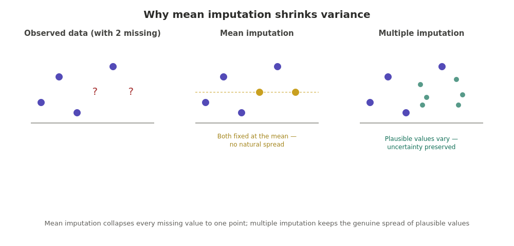
- Artificially reduces variance in the dataset, since every imputed value is identical and sits exactly at the center — this distorts standard deviation, confidence intervals, and any test relying on the data’s natural spread
- Distorts relationships (correlations) between variables, since the imputed values don’t reflect genuine covariation with other variables
- Widely considered a poor default choice in modern statistical practice, despite its historical popularity due to simplicity — mentioned here mainly because it remains common in introductory contexts, not because it’s recommended for serious analysis
Method 4: Regression Imputation
Use a regression model, built from the observed data, to predict what each missing value likely would have been, based on other variables in the dataset.
Worked example: Predicting missing income values using a regression model built on age, education level, and years of experience (all fully observed), then using each individual’s specific predicted value to fill their missing income.
Advantage: more sophisticated than mean imputation, since it uses relationships between variables rather than a single flat average.
Disadvantage: still tends to understate the true uncertainty in the data, since every imputed value falls exactly on the regression line, with no natural variability around the prediction — real observed data always has scatter around a regression line, but purely regression-imputed data doesn’t, again artificially shrinking variance.
Method 5: Multiple Imputation (The Modern Standard)
Rather than filling each missing value with a single “best guess,” multiple imputation creates several complete datasets (typically 20-100), each with the missing values filled in slightly differently, reflecting the genuine statistical uncertainty around what the true missing value might have been.
The process:
- Generate multiple (m) complete datasets, each imputing missing values using a model that includes random variation, not just a single point prediction
- Run the intended statistical analysis (e.g., a regression) separately on each of the m datasets
- Combine the m sets of results using Rubin’s Rules, which mathematically account for both the variability within each imputed dataset and the variability between the different imputed datasets
Why this solves the variance-shrinkage problem: because each of the m datasets imputes slightly different plausible values (drawing from a distribution rather than a single fixed prediction), the variation between the m datasets captures the genuine uncertainty about what the true missing values were — information that single imputation methods (mean or regression imputation) simply discard.
Disadvantage: considerably more computationally involved, and requires appropriate software (R’s mice package, Stata’s mi commands, or Python’s equivalents) rather than a simple manual calculation.
Method 6: Maximum Likelihood Estimation (Full Information Maximum Likelihood, FIML)
Rather than filling in missing values at all, FIML uses all available data directly to estimate model parameters, using the mathematical properties of the likelihood function to handle missingness without imputation.
Advantage: avoids the need to generate imputed datasets altogether, and produces statistically efficient estimates under MAR.
Disadvantage: requires specific statistical software capable of FIML estimation (common in structural equation modeling software), and the underlying mathematics is considerably more complex than the deletion or imputation methods above.
Choosing the Right Method: A Decision Framework
| Situation | Recommended approach |
|---|---|
| Very small amount of missing data (<5%), confirmed MCAR | Listwise deletion is often acceptable |
| Moderate missingness, MAR | Multiple imputation (preferred modern standard) |
| Data intended for structural equation modeling | FIML, if software supports it |
| Quick exploratory analysis, not for final reported results | Mean imputation may be acceptable as a rough first pass, with limitations clearly acknowledged |
| Suspected MNAR | No standard method fully solves this — consider sensitivity analysis, or explicit modeling of the missingness mechanism itself |
Common Student Mistakes
- Defaulting to mean imputation without considering its variance-shrinking effect — this remains one of the most common errors in student research projects, often chosen for its simplicity without acknowledging its statistical cost
- Assuming data is MCAR without checking — this assumption should be examined (e.g., comparing observed characteristics of cases with and without missing data), not simply assumed for convenience
- Treating imputed values as if they were genuinely observed — particularly in single imputation methods, forgetting that imputed values carry more uncertainty than real observations, and failing to account for this in reported confidence intervals
- Applying listwise deletion without checking how much data is actually lost — as shown in the worked example, missingness across multiple variables can compound into a much larger data loss than expected
If you need academic support with missing-data analysis, statistical methods, or a data analytics assignment, you can explore our Data Analytics Assignment Help
Frequently Asked Questions
How much missing data is “too much” to analyze reliably? There’s no universal cutoff, but many researchers treat missingness above roughly 10% per variable as warranting serious consideration of imputation methods rather than simple deletion — the appropriate threshold also depends heavily on the missingness mechanism (MCAR vs MAR vs MNAR), not just the raw percentage.
Is multiple imputation always better than single imputation methods? For most modern research purposes, yes — multiple imputation more accurately reflects the genuine uncertainty in missing data, whereas single imputation methods (mean, regression) tend to understate that uncertainty, producing overly narrow confidence intervals and potentially misleading statistical significance.
Can missing data ever be safely ignored? Only if it’s a very small proportion of the dataset and confirmed (not just assumed) to be MCAR — even then, transparency about how missingness was handled is expected in rigorous research reporting.
What software is commonly used for multiple imputation? R’s mice package and Stata’s built-in mi commands are widely used in academic research; Python’s scikit-learn and statsmodels ecosystems also offer imputation tools, though historically with somewhat less specialized support for multiple imputation specifically compared to R and Stata.