Data Cleaning and Preprocessing: A Step-by-Step Guide for Analysts

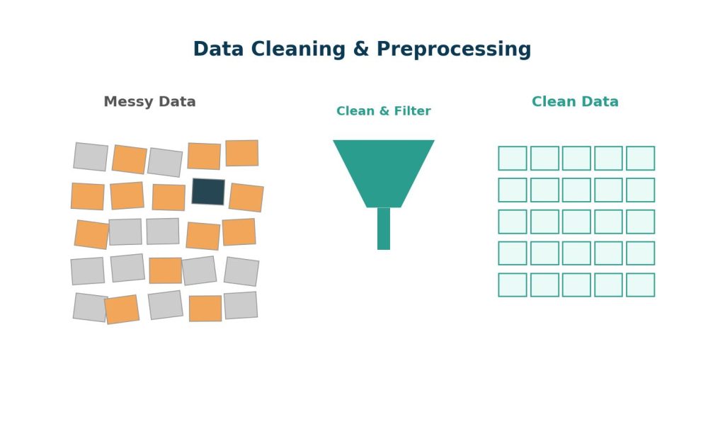
If descriptive statistics and machine learning models are the “engine” of data analytics, data cleaning is the fuel refinement process — unglamorous, but absolutely essential. Analysts and data scientists routinely report spending 60–80% of their project time cleaning and preparing data rather than analyzing it. For students in a data analytics course, mastering this skill is arguably more valuable in the short term than mastering any single statistical technique, because poor data quality silently invalidates even the most sophisticated analysis.

This article provides a structured, step-by-step guide to data cleaning and preprocessing, with worked examples in both SQL and Python (pandas).

Why Data Cleaning Matters: Garbage In, Garbage Out

The principle of “garbage in, garbage out” (GIGO) is central to data analytics. A regression model built on data with unaddressed outliers, inconsistent units, or systematically missing values will produce confident-looking but incorrect conclusions. Real-world consequences of poor data quality include:

• A healthcare model that under-predicts risk for a patient group due to missing records concentrated in that group.
• A retail forecast that overestimates demand because duplicate transactions inflated historical sales figures.
• A marketing analysis that misattributes revenue because currency values weren’t standardized across regions.

Step 1: Understand the Data Before Touching It

Before cleaning anything, analysts perform an initial data audit:

• Check the shape: How many rows and columns?
• Check data types: Are dates stored as text? Are numeric fields stored as strings?
• Check summary statistics: .describe() in pandas quickly reveals implausible values (e.g., a negative age, or a maximum order value of $9,999,999).
• Check for duplicates and missingness: .isnull().sum() and .duplicated().sum() in pandas.

import pandas as pd

df = pd.read_csv("orders.csv")
print(df.shape)
print(df.dtypes)
print(df.describe())
print(df.isnull().sum())
print(df.duplicated().sum())

Step 2: Handle Missing Data

Missing data is one of the most common and consequential data quality issues (for a deeper statistical treatment, see How to Handle Missing Data in Statistical Analysis: Methods Compared). There are three broad strategies:

1. Deletion — Remove rows or columns with missing values. Appropriate when missingness is small (e.g., under 5%) and appears random.
2. Imputation — Fill missing values using the mean, median, mode, or a model-based estimate. Appropriate when deletion would lose too much data.
3. Flagging — Create a new binary column indicating whether a value was missing, preserving the information that missingness itself might be meaningful.

Worked example: A dataset of 10,000 customer records has 400 missing “annual income” values (4%). Checking further, the analyst finds these are concentrated among customers who signed up via a specific mobile app version that had a form bug — meaning the missingness is not random (it’s “missing not at random,” or MNAR). Rather than filling these with the column mean (which would bias the income distribution), the analyst chooses to impute using the median income within the customer’s zip code, a more contextually accurate estimate, and adds a flag column income_was_imputed so downstream models can account for the uncertainty.

# Median imputation grouped by a related column
df["annual_income"] = df.groupby("zip_code")["annual_income"].transform(
    lambda x: x.fillna(x.median())
)
df["income_was_imputed"] = df["annual_income"].isna()

Step 3: Remove or Resolve Duplicates

Duplicate records inflate counts and skew aggregate statistics. Duplicates can be exact (identical rows) or “fuzzy” (e.g., “Jon Smith” vs. “Jonathan Smith” referring to the same customer).

# Exact duplicates
df = df.drop_duplicates()

# Duplicates based on a subset of columns (e.g., same order ID logged twice)
df = df.drop_duplicates(subset=["order_id"], keep="first")

In SQL, a common pattern to identify duplicates is:

SELECT order_id, COUNT(*) AS occurrences
FROM orders
GROUP BY order_id
HAVING COUNT(*) > 1;

Worked example: QuickBite’s order database shows 2.31 million rows, but a check reveals 14,000 order IDs appear twice due to a retry bug in the checkout API that occasionally double-logged successful orders. Removing these duplicates reduces total revenue calculations by roughly $210,000 — a correction that materially changes quarterly reporting.

Step 4: Detect and Handle Outliers

Outliers are extreme values that may represent genuine rare events, measurement errors, or data entry mistakes. Common detection methods include:

• Z-score method: Flag values more than 3 standard deviations from the mean (assumes roughly normal distribution).
• IQR (Interquartile Range) method: Flag values below Q1 − 1.5×IQR or above Q3 + 1.5×IQR — more robust to skewed distributions.
• Visual inspection: Box plots and scatter plots often reveal outliers a summary statistic would miss.

Q1 = df["order_value"].quantile(0.25)
Q3 = df["order_value"].quantile(0.75)
IQR = Q3 - Q1
lower_bound = Q1 - 1.5 * IQR
upper_bound = Q3 + 1.5 * IQR

outliers = df[(df["order_value"] < lower_bound) | (df["order_value"] > upper_bound)]
print(f"Found {len(outliers)} outlier orders")

Worked example: In QuickBite’s order data, the IQR method flags 340 orders with a value above $500 — unusual for a food delivery app where the typical order is $18–$35. Investigating further, the analyst finds these are legitimate bulk catering orders, not errors. Rather than deleting them, the analyst creates a separate order_type category (“catering” vs. “standard”) so these orders don’t distort the typical customer’s average order value calculation.

This example illustrates an important principle: not all outliers should be removed. The correct action depends on whether the outlier reflects a genuine, meaningful data point or an error.

Step 5: Standardize Formats and Units

Inconsistent formatting is a frequent source of hidden errors, especially in datasets combined from multiple sources.

• Dates: Ensure all dates use a single format (e.g., ISO 8601: YYYY-MM-DD) and time zone.
• Text case: Standardize categorical text (e.g., “NY”, “New York”, “new york” should all map to one value).
• Units: Ensure currency, weight, or distance fields use consistent units (e.g., all revenue in USD, not a mix of USD and local currency).

df["state"] = df["state"].str.strip().str.upper()
df["order_date"] = pd.to_datetime(df["order_date"], errors="coerce")

Step 6: Encode Categorical Variables (for Modeling)

If the cleaned data will feed into a statistical or machine learning model, categorical variables often need to be converted into numeric form:

• One-hot encoding: Creates a separate binary column for each category (best for nominal data with no inherent order, like restaurant cuisine type).
• Label/ordinal encoding: Assigns an integer to each category (appropriate only when categories have a natural order, like “low,” “medium,” “high” satisfaction ratings).

df_encoded = pd.get_dummies(df, columns=["cuisine_type"], drop_first=True)

Step 7: Normalize or Scale Numeric Features

Many statistical and machine learning algorithms (e.g., k-nearest neighbors, gradient descent-based models) are sensitive to the scale of input variables. Two common techniques:

• Min-Max normalization: Rescales values to a 0–1 range.
• Standardization (Z-score scaling): Rescales values to have a mean of 0 and standard deviation of 1.

from sklearn.preprocessing import StandardScaler

scaler = StandardScaler()
df[["order_value_scaled"]] = scaler.fit_transform(df[["order_value"]])

Building a Data Cleaning Checklist

A practical checklist students can apply to any new dataset:

1. Inspect shape, data types, and summary statistics.
2. Identify and handle missing values (delete, impute, or flag).
3. Identify and remove exact and fuzzy duplicates.
4. Detect outliers and decide whether to remove, cap, or retain them.
5. Standardize date formats, text casing, and units.
6. Encode categorical variables if preparing for modeling.
7. Scale or normalize numeric features if the chosen algorithm requires it.
8. Document every transformation made, so the cleaning process is reproducible. Once your checklist is complete, the natural next step is Exploratory Data Analysis (EDA): Techniques, Tools, and Worked Examples.

Students working on data cleaning and preprocessing for analytics coursework can also explore this Data Analytics Assignment Help resource for support with data analysis, Python, statistics, visualization, and related analytics projects.

FAQs

Q1: What percentage of missing data is “too much” to simply delete? There’s no universal threshold, but many practitioners treat under 5% missingness in a column as generally safe to delete (if missing completely at random), while higher percentages usually call for imputation or a deeper investigation into why the data is missing.

Q2: Should outliers always be removed? No. Outliers should be investigated before removal. Some represent genuine rare events (e.g., a legitimate bulk order) that carry real information, while others represent data entry errors that should be corrected or removed.

Q3: What is the difference between data cleaning and data preprocessing? Data cleaning typically refers to fixing errors and inconsistencies (missing values, duplicates, wrong formats), while data preprocessing is the broader term that includes cleaning plus additional steps needed to prepare data for modeling, such as encoding categorical variables and scaling numeric features.

Q4: Why does missingness sometimes need special handling instead of simple mean imputation? When data is “missing not at random” (MNAR) — meaning the fact that it’s missing is related to its actual value or another variable — simple mean imputation can introduce bias. Understanding why data is missing is as important as deciding how to fill it.

Q5: What tools are best for data cleaning? For small to medium datasets, Excel (see Excel for Data Analytics: Advanced Functions, Pivot Tables, and Dashboards) and Python’s pandas library (see Python vs R for Data Analysis: Which to Learn First) are the most common tools taught in university courses. For very large datasets, SQL and distributed frameworks like Apache Spark are used. OpenRefine is also popular for cleaning messy, semi-structured data.

Q6: How do I know if my cleaning process is “good enough”? A useful test is reproducibility and transparency: could another analyst follow your documented steps and arrive at the same cleaned dataset? Additionally, compare summary statistics before and after cleaning to confirm the changes make sense and haven’t introduced new distortions.