
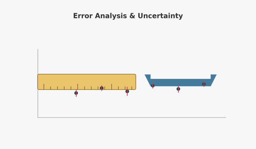
Of every section in a physics lab report, the uncertainty analysis is the one most students write last, rush through, and understand least — despite it often being weighted just as heavily as the experiment itself, whether that experiment is a kinematics timing trial or a more involved multi-step setup. Part of the problem is that “error” in physics doesn’t mean “mistake” the way it does in everyday language, and the propagation formulas feel like an entirely separate math topic bolted onto the physics. This guide clarifies what uncertainty actually represents, how to calculate and propagate it correctly, and how to report it properly — with worked examples throughout.
Table of Contents
Toggle“Error” Doesn’t Mean “Mistake”
In everyday language, an “error” implies something went wrong. In physics, error and uncertainty refer to the inherent limitations of any measurement — every measuring instrument has a finite precision, and every measured quantity carries some unavoidable uncertainty, even when the experiment is performed perfectly. Reporting uncertainty isn’t admitting to a mistake; it’s a required, honest statement of how precisely you actually know a value.
Two distinct types of error worth distinguishing clearly in a lab report:
- Random error — causes scatter in repeated measurements, in both directions, due to unpredictable small variations (reading a scale slightly differently each time, small fluctuations in conditions). Reduced by taking more measurements and averaging.
- Systematic error — causes a consistent bias in one direction across all measurements (a scale that’s not zeroed correctly, a timer that consistently runs slightly fast). Not reduced by averaging more measurements — it requires identifying and correcting the source of the bias itself.
Worked example distinguishing the two: “If a stopwatch consistently starts 0.2 seconds late every trial, this introduces a systematic error — every measured time will be too short by roughly the same amount, no matter how many trials are averaged. If, instead, the person operating the stopwatch reacts slightly differently each time (sometimes a bit early, sometimes a bit late), this introduces random error, which averages out somewhat over many trials but still contributes to the spread of results.”
Reporting a Single Measurement’s Uncertainty
For a single measurement, uncertainty is typically estimated from the smallest division of the measuring instrument, often taken as half of the smallest marked increment (though conventions vary — always check your specific lab manual’s expectation).
Worked example: “A ruler marked in millimeters is used to measure a length of 15.3 cm. Since the smallest division is 1 mm (0.1 cm), the estimated uncertainty is typically taken as half of that smallest division: ±0.05 cm. The measurement would be reported as 15.30 ± 0.05 cm.”
Calculating Uncertainty From Repeated Measurements
When a measurement is repeated multiple times, uncertainty is calculated statistically, using the mean and standard deviation.
Mean: x̄ = (Σxᵢ) / n
Standard deviation: s = √[Σ(xᵢ − x̄)² / (n − 1)]
Standard error of the mean (often what’s actually reported as the final uncertainty): SEM = s / √n
Worked example: Five trials measuring the period of a pendulum give: 2.01 s, 1.98 s, 2.03 s, 1.99 s, 2.04 s.
Step 1 — Calculate the mean: x̄ = (2.01 + 1.98 + 2.03 + 1.99 + 2.04) / 5 = 10.05 / 5 = 2.01 s
Step 2 — Calculate each deviation from the mean and square it: (2.01−2.01)² = 0 (1.98−2.01)² = 0.0009 (2.03−2.01)² = 0.0004 (1.99−2.01)² = 0.0004 (2.04−2.01)² = 0.0009 Sum = 0.0026
Step 3 — Calculate standard deviation: s = √(0.0026/4) = √0.00065 = 0.0255 s
Step 4 — Calculate standard error of the mean: SEM = 0.0255/√5 = 0.0255/2.236 = 0.0114 s
Answer: The period would be reported as 2.01 ± 0.01 s (rounding the uncertainty to match significant figures, discussed below).
Common mistake to avoid: Reporting the standard deviation itself as the final “uncertainty” without recognizing that the standard error of the mean (which accounts for the number of trials) is usually what’s expected when repeated trials are averaged — check your specific lab’s requirements, since conventions do vary between courses.
Propagating Uncertainty Through Calculations
Once you have uncertainties on individual measured quantities, you often need to combine them to find the uncertainty in a calculated result — this is called propagation of uncertainty, and it follows different rules depending on the mathematical operation involved.
Addition and Subtraction: Add the Absolute Uncertainties
If z = x + y (or z = x − y), then: δz = δx + δy (adding absolute uncertainties, regardless of whether the quantities themselves are added or subtracted)
Worked example: “Two lengths are measured as 12.5 ± 0.2 cm and 8.3 ± 0.1 cm. Find the uncertainty in their sum. Sum = 12.5 + 8.3 = 20.8 cm. Uncertainty: δz = 0.2 + 0.1 = 0.3 cm. Result: 20.8 ± 0.3 cm.”
Multiplication and Division: Add the Relative (Fractional) Uncertainties
If z = xy (or z = x/y), then: δz/z = √[(δx/x)² + (δy/y)²] (for independent uncertainties, using the more accurate “in quadrature” formula) — or, as a simpler, more conservative approximation often used in introductory courses: δz/z = δx/x + δy/y
Worked example (using the simpler addition approximation, common in intro labs): “A rectangle’s sides are measured as 5.0 ± 0.1 cm and 3.0 ± 0.1 cm. Find the area and its uncertainty.
Area = 5.0 × 3.0 = 15.0 cm²
Relative uncertainty in length: 0.1/5.0 = 0.02 (2%) Relative uncertainty in width: 0.1/3.0 = 0.033 (3.3%) Combined relative uncertainty: 0.02 + 0.033 = 0.053 (5.3%)
Absolute uncertainty in area: 0.053 × 15.0 = 0.8 cm²
Result: Area = 15.0 ± 0.8 cm²”
Common mistake to avoid: Adding the absolute uncertainties (0.1 + 0.1 = 0.2 cm) directly for a multiplication problem, treating it the same as an addition problem. Multiplication and division require converting to relative (fractional or percentage) uncertainty first, combining those, and then converting back to an absolute uncertainty for the final result — this is the single most common error in uncertainty propagation.
Powers: Multiply the Relative Uncertainty by the Exponent
If z = xⁿ, then: δz/z = n(δx/x)
Worked example: “The radius of a circle is measured as 4.0 ± 0.1 cm. Find the uncertainty in the calculated area (Area = πr²).
Area = π(4.0)² = 50.27 cm²
Relative uncertainty in r: 0.1/4.0 = 0.025 (2.5%) Since Area depends on r², the exponent is 2: relative uncertainty in Area = 2 × 0.025 = 0.05 (5%)
Absolute uncertainty in Area: 0.05 × 50.27 = 2.5 cm²
Result: Area = 50.3 ± 2.5 cm²”
Common mistake to avoid: Treating r² the same as multiplying two independently measured quantities (which would use the quadrature or addition rule for multiplication). Since r is the same measured quantity multiplied by itself, the power rule (multiply relative uncertainty by the exponent) applies instead — this distinction is a common point of confusion, since r × r looks superficially like a multiplication of two different quantities.
Significant Figures and Rounding Uncertainty
A commonly enforced (and commonly lost) rule: uncertainty values are typically rounded to one or two significant figures, and the measured value is then rounded to match the same decimal place as the uncertainty.
Worked example: “A calculation gives a result of 24.3768 with a calculated uncertainty of 0.3421. Round the uncertainty to one significant figure first: 0.3. Then round the main value to match the same decimal place: 24.4. Final reported result: 24.4 ± 0.3.”
Common mistake to avoid: Reporting an uncertainty with far more precision than the measurement itself justifies (such as ±0.3421), or reporting the main value with more decimal places than the uncertainty supports (such as 24.3768 ± 0.3, which implies false precision in the main value beyond what the uncertainty actually justifies).
Comparing Results Using Percent Error and Percent Difference
- Percent error (used when comparing to an accepted/theoretical value): % error = |experimental − accepted| / accepted × 100%
- Percent difference (used when comparing two experimental values, with no accepted “correct” value): % difference = |value₁ − value₂| / [(value₁ + value₂)/2] × 100%
Worked example: “An experiment measures the acceleration due to gravity as 9.65 m/s², compared to the accepted value of 9.81 m/s².
% error = |9.65 − 9.81| / 9.81 × 100% = 0.16/9.81 × 100% = 1.63%”
Common mistake to avoid: Using the percent error formula when comparing two experimentally measured values with no single “accepted” reference value — in that case, percent difference (using the average of the two values in the denominator) is the appropriate formula instead.
A Step-by-Step Checklist for Students Stuck on a Lab Report’s Uncertainty Section
- Distinguish clearly between random error (reduced by averaging) and systematic error (requires identifying and correcting the source) when discussing sources of uncertainty.
- For repeated measurements, calculate the mean, standard deviation, and standard error of the mean, checking your specific lab’s convention for which one to report as final uncertainty.
- For propagating uncertainty through calculations: use addition of absolute uncertainties for sums/differences, addition of relative uncertainties for products/quotients, and the power rule (multiply relative uncertainty by the exponent) for powers of a single measured quantity.
- Round your final uncertainty to one or two significant figures, then round your main result to match the same decimal place.
- Use percent error only when comparing to a known accepted value; use percent difference when comparing two experimental results with no accepted reference.
Need help applying uncertainty analysis to a physics assignment or lab report? If you’re working on a broader physics assignment involving experimental data, calculations, mechanics, waves, electricity, or other topics, you can explore our Physics Assignment Help service for academic support.
FAQs
Q1: What’s the difference between accuracy and precision in the context of error analysis? Accuracy describes how close a measurement is to the true or accepted value, while precision describes how consistent or reproducible repeated measurements are with each other, regardless of whether they’re close to the true value. A set of measurements can be precise (tightly clustered) but inaccurate (consistently off from the true value) if there’s a systematic error present.
Q2: Do I always use the “add in quadrature” formula or the simpler addition formula for propagating multiplicative uncertainty? This depends on your specific course’s expectations — the quadrature formula (square root of the sum of squares) is more statistically accurate for independent, random uncertainties, while simple addition of relative uncertainties is a more conservative, simpler approximation often used in introductory labs. Always check your lab manual or ask your instructor which convention is expected.
Q3: Why can’t systematic error be reduced just by taking more measurements? Because systematic error introduces a consistent bias in the same direction every time — averaging more measurements only reduces the effect of random scatter, not a bias that shifts every single measurement in the same direction by roughly the same amount. Correcting systematic error requires identifying its actual source (like recalibrating an instrument) rather than statistical averaging.
Q4: How many significant figures should my final answer have? As a general rule, your final uncertainty should be rounded to one or two significant figures, and your main measured or calculated value should then be rounded to match the same decimal place as that uncertainty — reporting more decimal places in your main value than your uncertainty justifies implies a false sense of precision.
Q5: What should I do if my percent error is very high — does that mean my experiment failed? Not necessarily — a high percent error is useful, honest data that should prompt a genuine discussion in your lab report about likely sources of systematic error (equipment calibration, simplifying assumptions, environmental factors) rather than being hidden or dismissed. A thoughtful discussion of a large discrepancy often earns more credit than an unrealistically small one that isn’t adequately explained.
Q6: Which topics is this uncertainty analysis most often applied to? Any lab measuring a quantity from wave interference or diffraction — slit spacing, fringe position, wavelength — will need exactly this propagation treatment, since those calculations chain together several measured quantities. The same applies to a circuit lab measuring current or resistance, where component tolerances and meter precision both need to be propagated into a final reported uncertainty.